1.1 什么是数据结构？

在计算机世界中，数据结构代表了计算机在内存中存储和组织数据的独特方法。通过不同的排列和组合方式，可以使用户高效且适当的方式访问和使用他们所需的数据。
数据结构的存在使用户能够方便地按需访问和操作他们的数据，有助于以高效而紧凑的方式组织和检索各种类型的数据。

对于接触过计算机基础知识的读者而言，对于下面这个公式应该不会陌生：

算法 + 数据结构 = 程序

提出这一公式并以此作为其一本专著书名Algorithms + Data Structures = Programs的瑞士计算机科学家Niklaus Wirth于1984年获得了图灵奖。

程序（Program）是由数据结构（Data Structure）和算法（Algorithm）组成，这意味着的程序的好和快是直接由程序所采用的数据结构和算法决定的。

❗️ 注意
本章节仅作介绍，涉及到的具体数据结构和算法会在后续章节中详细讲解。

数据结构分类

数据也可以被细分为以下两种类型：

线性结构
非线性结构

线性结构

数据元素按顺序或者线性排列
除了第一个元素和最后一个元素之外，剩余每个元素都有前一个和下一个相邻元素。

有两种技术可以在内存中表示这种线性结构。

数组：存储在连续内存位置的相同数据类型的项目的集合。
链表：通过使用指针或链接的概念来表示的所有元素之间的线性关系。

常见的线性结构例子有：

数组：存储在连续内存位置的元素的集合。
链表：节点的集合，每个节点包含一个元素和对下一个节点的引用。
堆栈：具有后进先出 (LIFO)顺序的元素集合。
队列：具有先进先出 (FIFO)顺序的元素集合。

非线性结构

该结构主要用于表示包含各种元素之间的层次关系的数据。

常见的非线性结构例子有：

图：顶点（节点）和表示顶点之间关系的边的集合。图用于建模和分析网络，例如社交网络或交通网络。
树：树的结构呈现出一个类似根和分支的形状，其中有一个根节点，从根节点出发，分成多个子节点，每个子节点可以又分为更多的子节点，依此类推

各种数据结构的简单介绍

数组（Arrays）

数组是相似数据元素的集合。这些数据元素具有相同的数据类型。
数组的元素存储在连续的内存位置中，并由索引（也称为下标）来指向数据。

在C语言中，数组声明使用以下格式：

ElemType name[size];
//例如
char array[10] = {'A', 'B', 'C', 'D', 'E', 'F', 'G', 'H', 'I', 'J'
// 完整代码：https://totuma.cn

上面的语句声明了一个包含10个元素的数组标记。在C中，数组索引从零开始。这意味着数组标记将总共包含10个元素。

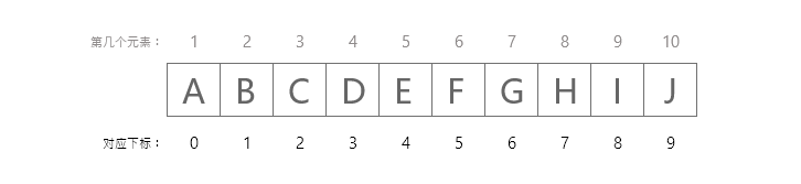
数组下标对应位序

第一个元素将存储在array[0]中，第二个元素将存储在array[1]中，等等。因此，最后一个元素，即第10个元素，将被存储在array[9]中。 在计算机中存储如下图所示。

当我们想要存储大量相同类型的数据时，通常会使用数组。当然，数组也有一些限制，比如：

数组的大小是固定的。
数据元素存储在连续的内存位置中，但是内存中剩余的大小可能不足以容纳当前数组。
元素的插入和删除会很麻烦。

链表（Linked Lists）

链表是一种非常灵活的动态数据结构，其中元素（称为节点）形成一个顺序列表。与静态数组相比，我们不需要担心链表中将存储多少个元素。这个特性使我们能够编写需要较少维护的健壮程序。在链表中，每个节点都有data域和next指针域：

data域：存放该节点或与该节点对应的任何其他数据的值。
next指针域：指向列表中的下一个节点的指针或链接。

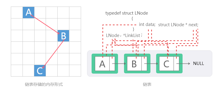
链表结构

列表中的最后一个节点包含一个NULL指针，表明它是当前列表的尾。由于节点的内存是在添加到列表中时动态分配的，因此可以添加到列表中的节点总数仅受可用内存量的限制。具体结构可见下图：

栈（Stacks）

栈是一种线性数据结构，其中元素的插入和删除只在一端完成，这被称为栈顶。栈被称为先入后出（LIFO）结构，因为添加到堆栈中的最后一个元素是从堆栈中删除的第一个元素。在计算机的内存中，堆栈可以使用数组或链表来实现。
下面可视化操作显示了一个栈的数组实现。每个栈都有一个与其关联的变量top，用于指向最上面的元素。这是将从中添加或删除元素的位置。

栈支持push 入栈和pop 出栈 操作，push 就是在从栈顶中压入一个元素，pop 就是在栈顶中弹出一个元素，即增和删。

💡 提示
点击下方的入栈、出栈按钮。可以明了的理解到什么是先入后出。

栈 | 可视化完整可视化

1.1 What is a Data Structure? - Data Structures Tutorial Visualize your code with animations

什么是堆栈？

堆栈是一种线性数据结构，其中新元素的插入和现有元素的删除发生在表示为堆栈顶部的同一端。

为了实现栈，需要维护一个 指向栈顶的指针 ，栈顶是最后插入的元素，因为 我们只能访问栈顶的元素。

LIFO（后进先出）：

该策略规定最后插入的元素将首先出现。您可以将一堆相互叠放的盘子作为现实生活中的示例。我们最后放置的盘子位于顶部，并且由于我们移除了顶部的盘子，所以我们可以说最后放置的盘子最先出现。

堆栈的基本操作

为了在堆栈中进行操作，向我们提供了某些操作。

push() 将一个元素插入栈中
pop() 从堆栈中删除一个元素
top() 返回栈顶元素。
如果堆栈为空， isEmpty()返回 true，否则返回 false。
size() 返回堆栈的大小。

堆

推：

将一个项目添加到堆栈中。如果堆栈已满，则称为 溢出情况。

推送算法：

开始
如果堆栈已满
返回
万一
别的  
增量顶部
stack[top] 赋值
结束其他
结束程序

流行音乐：

从堆栈中删除一个项目。项目的弹出顺序与推送顺序相反。如果堆栈为空，则称为下溢 条件。

流行算法：

开始
如果堆栈为空
返回
万一
别的
存储堆栈的值[top]
减少顶部
返回值
结束其他
结束程序

顶部：

返回栈顶元素。

顶部算法：

开始
返回堆栈[顶部]
结束程序

是空的：

如果堆栈为空则返回 true，否则返回 false。

isEmpty 的算法 ：

开始
如果顶部 < 1
返回真
别的
返回错误
结束程序

实际理解堆栈：

现实生活中有很多堆栈的例子。考虑一个简单的例子，在食堂里，盘子一个一个地叠在一起。位于顶部的盘子是第一个被移除的盘子，即放置在最底部位置的盘子在堆叠中保留最长的时间。因此，可以简单地看出遵循 LIFO/FILO 顺序。

复杂度分析：

时间复杂度

运营	复杂
推（）	复杂度(1)
流行音乐（）	复杂度(1)
是空的（）	复杂度(1)
尺寸（）	复杂度(1)

堆栈类型：

固定大小堆栈 ：顾名思义，固定大小堆栈具有固定的大小，不能动态增长或收缩。如果堆栈已满并尝试向其中添加元素，则会发生溢出错误。如果堆栈为空并且尝试从中删除元素，则会发生下溢错误。
动态大小堆栈 ：动态大小堆栈可以动态增长或收缩。当堆栈已满时，它会自动增加其大小以容纳新元素，而当堆栈为空时，它会减少其大小。这种类型的堆栈是使用链表实现的，因为它允许轻松调整堆栈的大小。

除了这两种主要类型之外，堆栈还有其他几种变体，包括：

中缀到后缀堆栈 ：这种类型的堆栈用于将中缀表达式转换为后缀表达式。
表达式计算堆栈 ：这种类型的堆栈用于计算后缀表达式。
递归堆栈 ：这种类型的堆栈用于跟踪计算机程序中的函数调用，并在函数返回时将控制权返回到正确的函数。
内存管理堆栈 ：这种类型的堆栈用于存储计算机程序中程序计数器的值和寄存器的值，允许程序在函数返回时返回到先前的状态。
平衡括号堆栈 ：这种类型的堆栈用于检查表达式中括号的平衡。
撤消重做堆栈 ：这种类型的堆栈用于计算机程序中，允许用户撤消和重做操作。

栈的应用：

中缀到后缀 /前缀的转换
许多地方都有重做/撤消功能，例如编辑器、Photoshop。
网络浏览器中的前进和后退功能
用于许多算法，如汉诺塔、树遍历、股票跨度问题和直方图问题。
回溯是算法设计技术之一。回溯的一些例子包括骑士之旅问题、N-皇后问题、在迷宫中寻找出路以及所有这些问题中的类似国际象棋或西洋跳棋的问题，如果这种方式效率不高，我们会回到之前的问题状态并进入另一条道路。为了从当前状态返回，我们需要存储以前的状态，为此我们需要一个堆栈。
在拓扑排序和强连通分量等图算法中
在内存管理中，任何现代计算机都使用堆栈作为运行目的的主要管理。计算机系统中运行的每个程序都有自己的内存分配
字符串反转也是栈的另一个应用。这里每个字符都被一一插入到堆栈中。因此，字符串的第一个字符位于堆栈底部，字符串的最后一个元素位于堆栈顶部。在堆栈上执行弹出操作后，我们得到一个相反顺序的字符串。
堆栈还有助于在计算机中实现函数调用。最后调用的函数总是最先完成。
堆栈还用于在文本编辑器中实现撤消/重做操作。

堆栈的实现：

堆栈可以使用数组或链表来实现。在基于数组的实现中，推送操作是通过递增顶部元素的索引并将新元素存储在该索引处来实现的。弹出操作是通过递减顶部元素的索引并返回存储在该索引处的值来实现的。在基于链表的实现中，推送操作是通过使用新元素创建新节点并将当前顶节点的下一个指针设置为新节点来实现的。出栈操作是通过将当前顶节点的next指针设置为下一个节点并返回当前顶节点的值来实现的。

堆栈在计算机科学中通常用于各种应用，包括表达式求值、函数调用和内存管理。在表达式的计算中，堆栈可用于在处理操作数和运算符时存储它们。在函数调用中，堆栈可用于跟踪函数调用的顺序，并在函数返回时将控制权返回到正确的函数。在内存管理中，堆栈可用于存储计算机程序中的程序计数器的值和寄存器的值，从而允许程序在函数返回时返回到先前的状态。

总之，堆栈是一种按照 LIFO 原理运行的线性数据结构，可以使用数组或链表来实现。可以在堆栈上执行的基本操作包括入栈、出栈和查看，并且堆栈在计算机科学中常用于各种应用，包括表达式求值、函数调用和内存管理。有两种方法实现一个堆栈 –

使用数组
使用链表

使用数组实现堆栈：

C++

              
                
                    /* C++ program to implement basic stack 
   operations */
#include <bits/stdc++.h> 
  
using namespace std; 
  
#define MAX 1000 
  
class Stack { 
    int
                          top; 
  
public: 
    int
                          a[MAX]; // Maximum size of Stack 
                        
  
    Stack() { top = -1; } 
    bool push(int x); 
    int
                          pop(); 
    int
                          peek(); 
    bool isEmpty(); 
}; 
  
bool Stack::push(int x) 
{ 
    if
                          (top >= (MAX - 1)) { 
        cout << "Stack Overflow"; 
        return false; 
    } 
    else { 
        a[++top] = x; 
        cout << x << " pushed into stack\n"; 
        return true; 
    } 
} 
  
int Stack::pop() 
{ 
    if
                          (top < 0) { 
        cout << "Stack Underflow"; 
        return 0; 
    } 
    else { 
        int x = a[top--]; 
        return x; 
    } 
} 
int Stack::peek() 
{ 
    if
                          (top < 0) { 
        cout << "Stack is Empty"; 
        return 0; 
    } 
    else { 
        int x = a[top]; 
        return x; 
    } 
} 
  
bool Stack::isEmpty() 
{ 
    return (top < 0); 
} 
  
// Driver program to test above functions 
int main() 
{ 
    class Stack s; 
    s.push(10); 
    s.push(20); 
    s.push(30); 
    cout << s.pop() << " Popped from stack\n"; 
    
    //print top element of stack after popping 
    cout << "Top element is : " << s.peek() << endl; 
    
    //print all elements in stack : 
    cout <<"Elements present in stack : "; 
    while(!s.isEmpty()) 
    { 
        // print top element in stack 
        cout << s.peek() <<" "; 
        // remove top element in stack 
        s.pop(); 
    } 
  
    return 0; 
}

                  

              
            

C

              
                
                    // C program for array implementation of stack 
#include <limits.h> 
#include <stdio.h> 
#include <stdlib.h> 
  
// A structure to represent a stack 
struct Stack { 
    int
                          top; 
    unsigned capacity; 
    int* array; 
}; 
  
// function to create a stack of given capacity. It initializes size of 
                        
// stack as 0 
struct Stack* createStack(unsigned capacity) 
{ 
    struct Stack* stack = (struct Stack*)malloc(sizeof(struct Stack)); 
    stack->capacity = capacity; 
    stack->top = -1; 
    stack->array = (int*)malloc(stack->capacity * sizeof(int)); 
                        
    return stack; 
} 
  
// Stack is full when top is equal to the last index 
int isFull(struct Stack* stack) 
{ 
    return stack->top == stack->capacity - 1; 
} 
  
// Stack is empty when top is equal to -1 
int isEmpty(struct Stack* stack) 
{ 
    return stack->top == -1; 
} 
  
// Function to add an item to stack.  It increases top by 1 
                        
void push(struct Stack* stack, int item) 
{ 
    if
                          (isFull(stack)) 
        return; 
    stack->array[++stack->top] = item; 
    printf("%d pushed to stack\n", item); 
} 
  
// Function to remove an item from stack.  It decreases top by 1 
                        
int pop(struct Stack* stack) 
{ 
    if
                          (isEmpty(stack)) 
        return INT_MIN; 
    return stack->array[stack->top--]; 
} 
  
// Function to return the top from stack without removing it 
int peek(struct Stack* stack) 
{ 
    if
                          (isEmpty(stack)) 
        return INT_MIN; 
    return stack->array[stack->top]; 
} 
  
// Driver program to test above functions 
int main() 
{ 
    struct Stack* stack = createStack(100); 
  
    push(stack, 10); 
    push(stack, 20); 
    push(stack, 30); 
  
    printf("%d popped from stack\n", pop(stack)); 
                        
  
    return 0; 
} 

                  

              
            

Java

              
                
                    /* Java program to implement basic stack 
operations */
class Stack { 
    static
                          final int MAX = 1000; 
                        
    int
                          top; 
    int
                          a[] = new int[MAX]; // Maximum size of Stack 
  
    boolean
                          isEmpty() 
    { 
        return (top < 0); 
    } 
    Stack() 
                        
    { 
        top = -1; 
    } 
  
    boolean
                          push(int x) 
    { 
        if (top >= (MAX - 1)) { 
            System.out.println("Stack Overflow"); 
            return false; 
        } 
        else { 
            a[++top] = x; 
            System.out.println(x + " pushed into stack"); 
            return true; 
                        
        } 
    } 
  
    int
                          pop() 
    { 
        if (top < 0) { 
            System.out.println("Stack Underflow"); 
            return 0; 
                        
        } 
        else { 
            int x = a[top--]; 
            return x; 
        } 
    } 
  
    int
                          peek() 
    { 
        if (top < 0) { 
            System.out.println("Stack Underflow"); 
            return 0; 
                        
        } 
        else { 
            int x = a[top]; 
            return x; 
        } 
    } 
     
    void
                          print(){ 
    for(int i = top;i>-1;i--){ 
      System.out.print(" "+ a[i]); 
    } 
  } 
} 
  
// Driver code 
class Main { 
    public
                          static void main(String args[]) 
    { 
        Stack s = new Stack(); 
        s.push(10); 
                        
        s.push(20); 
                        
        s.push(30); 
                        
        System.out.println(s.pop() + " Popped from stack"); 
        System.out.println("Top element is :" + s.peek()); 
        System.out.print("Elements present in stack :"); 
        s.print(); 
    } 
} 

                  

              
            

Python3

              
                
                    # Python program for implementation of stack 
  
# import maxsize from sys module  
# Used to return -infinite when stack is empty 
from sys import maxsize 
  
# Function to create a stack. It initializes size of stack as 0 
                        
def createStack(): 
    stack = [] 
                        
    return
                          stack 
  
# Stack is empty when stack size is 0 
def isEmpty(stack): 
    return
                          len(stack) == 0
  
# Function to add an item to stack. It increases size by 1 
def push(stack, item): 
    stack.append(item) 
    print(item + " pushed to stack ") 
      
# Function to remove an item from stack. It decreases size by 1 
                        
def pop(stack): 
    if
                          (isEmpty(stack)): 
        return str(-maxsize -1) # return minus infinite 
      
    return
                          stack.pop() 
  
# Function to return the top from stack without removing it 
def peek(stack): 
    if
                          (isEmpty(stack)): 
        return str(-maxsize -1) # return minus infinite 
    return
                          stack[len(stack) - 1] 
  
# Driver program to test above functions     
                        
stack = createStack() 
push(stack, str(10)) 
push(stack, str(20)) 
push(stack, str(30)) 
print(pop(stack) + " popped from stack") 

                  

              
            

C#

              
                
                    // C# program to implement basic stack 
// operations 
using System; 
  
namespace ImplementStack { 
class Stack { 
    private
                          int[] ele; 
    private
                          int top; 
    private
                          int max; 
    public
                          Stack(int size) 
    { 
        ele = new int[size]; // Maximum size of Stack 
        top = -1; 
        max = size; 
    } 
  
    public
                          void push(int item) 
    { 
        if (top == max - 1) { 
            Console.WriteLine("Stack Overflow"); 
            return; 
        } 
        else { 
            ele[++top] = item; 
        } 
    } 
  
    public
                          int pop() 
    { 
        if (top == -1) { 
            Console.WriteLine("Stack is Empty"); 
            return -1; 
        } 
        else { 
            Console.WriteLine("{0} popped from stack ", ele[top]); 
            return ele[top--]; 
        } 
    } 
  
    public
                          int peek() 
    { 
        if (top == -1) { 
            Console.WriteLine("Stack is Empty"); 
            return -1; 
        } 
        else { 
            Console.WriteLine("{0} popped from stack ", ele[top]); 
            return ele[top]; 
        } 
    } 
  
    public
                          void printStack() 
    { 
        if (top == -1) { 
            Console.WriteLine("Stack is Empty"); 
            return; 
        } 
        else { 
            for (int
                          i = 0; i <= top; i++) { 
                Console.WriteLine("{0} pushed into stack", ele[i]); 
            } 
        } 
    } 
} 
  
// Driver program to test above functions 
class Program { 
    static
                          void Main() 
    { 
        Stack p = new Stack(5); 
  
        p.push(10); 
        p.push(20); 
        p.push(30); 
        p.printStack(); 
        p.pop(); 
    } 
} 
} 

                  

              
            

Javascript

              
                
                    <script> 
/* javascript program to implement basic stack 
operations  
*/
 var t = -1; 
      var MAX = 1000; 
    var
                          a = Array(MAX).fill(0); // Maximum size of Stack 
  
    function isEmpty() { 
        return (t < 0); 
    } 
  
    function push(x) { 
        if (t >= (MAX - 1)) { 
            document.write("Stack Overflow"); 
            return false; 
        } else { 
        t+=1; 
            a[t] = x; 
              
                        
            document.write(x + " pushed into stack<br/>"); 
            return true; 
                        
        } 
    } 
  
    function pop() { 
        if (t < 0) { 
            document.write("Stack Underflow"); 
            return 0; 
        } else { 
            var x = a[t]; 
            t-=1; 
            return x; 
        } 
    } 
  
    function peek() { 
        if (t < 0) { 
            document.write("Stack Underflow"); 
            return 0; 
        } else { 
            var x = a[t]; 
            return x; 
        } 
    } 
  
    function print() { 
        for (i = t; i > -1; i--) { 
            document.write(" " + a[i]); 
        } 
    } 
  
        push(10); 
        push(20); 
        push(30); 
        document.write(pop() + " Popped from stack"); 
        document.write("<br/>Top element is :" + peek()); 
                        
        document.write("<br/>Elements present in stack : "); 
        print(); 
  
// This code is contributed by Rajput-Ji  
</script> 

                  

              
            

输出

10 入栈
20 入栈
30 压入堆栈
30 从堆栈中弹出
顶部元素是：20
堆栈中存在的元素：20 10

数组实现的优点：

易于实施。
由于不涉及指针，因此节省了内存。

数组实现的缺点：

它不是动态的，即它不会根据运行时的需要而增长和收缩。 [但是对于动态大小的数组，例如 C++ 中的向量、Python 中的列表、Java 中的 ArrayList，堆栈也可以随着数组实现而增长和收缩]。
堆栈的总大小必须事先定义。

使用链表实现堆栈：

C++

              
                
                    // C++ program for linked list implementation of stack 
#include <bits/stdc++.h> 
using namespace std; 
  
// A structure to represent a stack 
class StackNode { 
public: 
    int
                          data; 
    StackNode* next; 
}; 
  
StackNode* newNode(int data) 
{ 
    StackNode* stackNode = new StackNode(); 
    stackNode->data = data; 
    stackNode->next = NULL; 
    return stackNode; 
} 
  
int isEmpty(StackNode* root) 
{ 
    return !root; 
} 
  
void push(StackNode** root, int data) 
{ 
    StackNode* stackNode = newNode(data); 
    stackNode->next = *root; 
    *root = stackNode; 
    cout << data << " pushed to stack\n"; 
} 
  
int pop(StackNode** root) 
{ 
    if
                          (isEmpty(*root)) 
        return INT_MIN; 
    StackNode* temp = *root; 
    *root = (*root)->next; 
    int
                          popped = temp->data; 
    free(temp); 
  
    return popped; 
} 
  
int peek(StackNode* root) 
{ 
    if
                          (isEmpty(root)) 
        return INT_MIN; 
    return root->data; 
} 
  
// Driver code 
int main() 
{ 
    StackNode* root = NULL; 
  
    push(&root, 10); 
    push(&root, 20); 
    push(&root, 30); 
  
    cout << pop(&root) << " popped from stack\n"; 
  
    cout << "Top element is " << peek(root) << endl; 
      
    cout <<"Elements present in stack : "; 
     //print all elements in stack : 
    while(!isEmpty(root)) 
    { 
        // print top element in stack 
        cout << peek(root) <<" "; 
        // remove top element in stack 
        pop(&root); 
    } 
  
    return 0; 
} 
  
// This is code is contributed by rathbhupendra 

                  

              
            

C

              
                
                    // C program for linked list implementation of stack 
#include <limits.h> 
#include <stdio.h> 
#include <stdlib.h> 
  
// A structure to represent a stack 
struct StackNode { 
    int
                          data; 
    struct StackNode* next; 
}; 
  
struct StackNode* newNode(int data) 
{ 
    struct StackNode* stackNode =  
                        
      (struct StackNode*) 
      malloc(sizeof(struct StackNode)); 
    stackNode->data = data; 
    stackNode->next = NULL; 
    return stackNode; 
} 
  
int isEmpty(struct StackNode* root) 
{ 
    return !root; 
} 
  
void push(struct StackNode** root, int data) 
{ 
    struct StackNode* stackNode = newNode(data); 
    stackNode->next = *root; 
    *root = stackNode; 
    printf("%d pushed to stack\n", data); 
} 
  
int pop(struct StackNode** root) 
{ 
    if
                          (isEmpty(*root)) 
        return INT_MIN; 
    struct StackNode* temp = *root; 
                        
    *root = (*root)->next; 
    int
                          popped = temp->data; 
    free(temp); 
  
    return popped; 
} 
  
int peek(struct StackNode* root) 
{ 
    if
                          (isEmpty(root)) 
        return INT_MIN; 
    return root->data; 
} 
  
int main() 
{ 
    struct StackNode* root = NULL; 
  
    push(&root, 10); 
    push(&root, 20); 
    push(&root, 30); 
  
    printf("%d popped from stack\n", pop(&root)); 
                        
  
    printf("Top element is %d\n", peek(root)); 
  
    return 0; 
} 

                  

              
            

Java

              
                
                    // Java Code for Linked List Implementation 
  
public class StackAsLinkedList { 
  
    StackNode root; 
  
    static
                          class StackNode { 
        int data; 
        StackNode next; 
  
        StackNode(int data) { this.data = data; } 
    } 
  
    public
                          boolean isEmpty() 
    { 
        if (root == null) { 
            return true; 
                        
        } 
        else
            return false; 
    } 
  
    public
                          void push(int data) 
    { 
        StackNode newNode = new StackNode(data); 
  
        if (root == null) { 
            root = newNode; 
        } 
        else { 
            StackNode temp = root; 
            root = newNode; 
            newNode.next = temp; 
        } 
        System.out.println(data + " pushed to stack"); 
    } 
  
    public
                          int pop() 
    { 
        int popped = Integer.MIN_VALUE; 
        if (root == null) { 
            System.out.println("Stack is Empty"); 
        } 
        else { 
            popped = root.data; 
            root = root.next; 
        } 
        return popped; 
    } 
  
    public
                          int peek() 
    { 
        if (root == null) { 
            System.out.println("Stack is empty"); 
            return Integer.MIN_VALUE; 
        } 
        else { 
            return root.data; 
        } 
    } 
  
    // Driver code 
    public
                          static void main(String[] args) 
    { 
  
        StackAsLinkedList sll = new StackAsLinkedList(); 
  
        sll.push(10); 
                        
        sll.push(20); 
                        
        sll.push(30); 
                        
  
        System.out.println(sll.pop() 
                           + " popped from stack"); 
  
        System.out.println("Top element is " + sll.peek()); 
    } 
}

                  

              
            

Python3

              
                
                    # Python program for linked list implementation of stack 
  
# Class to represent a node 
                        
  
  
class StackNode: 
  
    # Constructor to initialize a node 
    def
                          __init__(self, data): 
        self.data =
                          data 
        self.next
                          = None
  
  
class Stack: 
  
    # Constructor to initialize the root of linked list 
    def
                          __init__(self): 
        self.root =
                          None
  
    def
                          isEmpty(self): 
        return True if self.root is None
                          else False
  
    def
                          push(self, data): 
        newNode = StackNode(data) 
        newNode.next = self.root 
                        
        self.root =
                          newNode 
        print ("% d pushed to stack" % (data)) 
  
    def
                          pop(self): 
                        
        if (self.isEmpty()): 
            return float("-inf") 
        temp = self.root 
        self.root =
                          self.root.next
        popped = temp.data 
        return popped 
  
    def
                          peek(self): 
                        
        if self.isEmpty(): 
            return float("-inf") 
        return self.root.data 
  
  
# Driver code 
stack = Stack() 
stack.push(10) 
stack.push(20) 
stack.push(30) 
  
print ("% d popped from stack" % (stack.pop())) 
print ("Top element is % d " % (stack.peek())) 
  
# This code is contributed by Nikhil Kumar Singh(nickzuck_007) 
                        

                  

              
            

C#

              
                
                    // C# Code for Linked List Implementation 
using System; 
  
public class StackAsLinkedList { 
  
    StackNode root; 
  
    public
                          class StackNode { 
        public int data; 
        public StackNode next; 
  
        public StackNode(int data) { this.data = data; } 
    } 
  
    public
                          bool isEmpty() 
    { 
        if (root == null) { 
            return true; 
                        
        } 
        else
            return false; 
    } 
  
    public
                          void push(int data) 
    { 
        StackNode newNode = new StackNode(data); 
  
        if (root == null) { 
            root = newNode; 
        } 
        else { 
            StackNode temp = root; 
            root = newNode; 
            newNode.next = temp; 
        } 
        Console.WriteLine(data + " pushed to stack"); 
    } 
  
    public
                          int pop() 
    { 
        int popped = int.MinValue; 
        if (root == null) { 
            Console.WriteLine("Stack is Empty"); 
        } 
        else { 
            popped = root.data; 
            root = root.next; 
        } 
        return popped; 
    } 
  
    public
                          int peek() 
    { 
        if (root == null) { 
            Console.WriteLine("Stack is empty"); 
            return int.MinValue; 
        } 
        else { 
            return root.data; 
        } 
    } 
  
    // Driver code 
    public
                          static void Main(String[] args) 
    { 
  
        StackAsLinkedList sll = new StackAsLinkedList(); 
  
        sll.push(10); 
        sll.push(20); 
        sll.push(30); 
  
        Console.WriteLine(sll.pop() + " popped from stack"); 
  
        Console.WriteLine("Top element is " + sll.peek()); 
    } 
} 
  
/* This code contributed by PrinciRaj1992 */

                  

              
            

Javascript

              
                
                    <script> 
// javascript Code for Linked List Implementation 
  
var root; 
  
     class StackNode { 
  
        constructor(data) { 
            this.data = data; 
            this.next = null; 
        } 
    } 
  
     function isEmpty() { 
        if (root == null) { 
            return true; 
                        
        } else
            return false; 
    } 
  
     function push(data) { 
        var newNode = new StackNode(data); 
  
        if (root == null) { 
            root = newNode; 
        } else { 
            var temp = root; 
            root = newNode; 
            newNode.next = temp; 
        } 
        document.write(data + " pushed to stack<br/>"); 
    } 
  
     function pop() { 
        var popped = Number.MIN_VALUE; 
        if (root == null) { 
            document.write("Stack is Empty"); 
        } else { 
            popped = root.data; 
            root = root.next; 
        } 
        return popped; 
    } 
  
     function peek() { 
        if (root == null) { 
            document.write("Stack is empty"); 
            return Number.MIN_VALUE; 
        } else { 
            return root.data; 
        } 
    } 
  
    // Driver code 
        push(10); 
        push(20); 
        push(30); 
  
        document.write(pop() + " popped from stack<br/>"); 
  
        document.write("Top element is " + peek()); 
  
// This code is contributed by Rajput-Ji  
</script> 

                  

              
            

输出

10 压入堆栈
20 压入堆栈
30 压入堆栈
30 从堆栈中弹出
顶部元素为 20
堆栈中存在的元素：20 10

链表实现的优点：

堆栈的链表实现可以根据运行时的需要进行增长和收缩。
它被用在许多虚拟机中，比如 JVM。

链表实现的缺点：

由于涉及指针，需要额外的内存。
堆栈中不可能进行随机访问。

相关文章：

使用单链表实现堆栈
堆栈的应用、优点和缺点

队列（Queues）

队列是一种先进先出（FIFO）的数据结构，其中首先插入的元素是第一个要取出的元素。队列中的元素在队尾添加，然后在队头删除。与栈一样，队列也可以通过使用数组或链表来实现。每个队列都有队头和队尾，分别指向可以进行删除和插入的位置。

队列 | 可视化完整可视化

1.1 What is a Data Structure? - Data Structures Tutorial Visualize your code with animations

与Stack 类似， Queue 是一种线性数据结构，遵循特定的顺序执行存储数据的操作。顺序是先进先出 （FIFO） 。

人们可以将队列想象成一队人从队列的开头开始按顺序等待接收某些东西。它是一个有序列表，其中插入是在一端（称为后部）完成的，删除是从另一端（称为前部）完成的。队列的一个很好的例子是资源的任何消费者队列，其中先到达的消费者首先得到服务。
栈和队列的区别在于删除。在堆栈中，我们删除最近添加的项目；在队列中，我们删除最近最少添加的项目。

队列数据结构

队列的基本操作：

enqueue()： 将一个元素插入到队列的末尾，即后端。
dequeue()： 此操作删除并返回位于队列前端的元素。
front()： 该操作返回前端的元素，但不删除它。
after()： 该操作返回后端的元素，但不删除它。
isEmpty()： 该操作指示队列是否为空。
isFull()： 该操作指示队列是否已满。
size()： 此操作返回队列的大小，即队列包含的元素总数。

队列类型：

简单队列： 简单队列也称为线性队列，是队列的最基本版本。这里，插入元素即入队操作发生在后端，移除元素即出队操作发生在前端。这里的问题是，如果我们从前面弹出一些项目，然后后面达到队列的容量，虽然前面有空白意味着队列未满，但根据 isFull() 函数中的条件，它将显示那么队列已满。为了解决这个问题我们使用循环队列。
循环队列 ：在循环队列中，队列的元素充当圆环。循环队列的工作原理与线性队列类似，只是最后一个元素连接到第一个元素。它的优点是可以更好地利用内存。这是因为如果存在空白空间，即如果队列中的某个位置不存在元素，则可以使用模容量（%n）轻松地在该位置添加元素。
优先队列 ：该队列是一种特殊类型的队列。它的特点是它根据某种优先级排列队列中的元素。优先级可以是具有最高值的元素具有优先级，因此它创建一个按值降序排列的队列。优先级也可以是具有最低值的元素获得最高优先级，因此它依次创建一个值顺序递增的队列。在预定义优先级队列中，C++优先考虑最高值，而Java优先考虑最低值。
出队：出队也称为双端队列。顾名思义，双端队列意味着可以从队列的两端插入或删除一个元素，这与其他队列只能从一端插入或删除元素不同。由于此属性，它可能不遵守先进先出属性。

队列的应用：

当事物不需要立即处理，但必须像广度优先搜索那样以先入先出的顺序处理时，就会使用队列。队列的这一属性使其在以下场景中也很有用。

当资源在多个消费者之间共享时。示例包括 CPU 调度、磁盘调度。
当数据在两个进程之间异步传输时（数据接收速率不一定与发送速率相同）。示例包括 IO 缓冲区、管道、文件 IO 等。
队列可以用作各种其他数据结构的重要组成部分。

队列的数组实现：

为了实现队列，我们需要跟踪两个索引：前索引和后索引。我们在后面将一个项目入队，并从前面将一个项目出队。如果我们只是简单地增加前部和后部索引，那么可能会出现问题，前部可能会到达数组的末尾。解决这个问题的办法就是以循环的方式增加前后。

入队步骤：

检查队列是否已满
如果已满，则打印溢出并退出
如果队列未满，则增加tail并添加元素

出队步骤：

检查队列是否为空
如果为空，则打印下溢并退出
如果不为空，则打印头部元素并增加头部

下面是一个在队列上实现上述操作的程序

C++

              
                
                    // CPP program for array
                        
// implementation of queue
                        
#include <bits/stdc++.h>
using namespace std;
 
// A structure to represent a queue
class Queue {
public:
    int
                          front, rear, size;
    unsigned capacity;
    int* array;
};
 
// function to create a queue
// of given capacity.
                        
// It initializes size of queue as 0
Queue* createQueue(unsigned capacity)
{
    Queue* queue = new Queue();
    queue->capacity = capacity;
    queue->front = queue->size = 0;
 
    // This is important, see the enqueue
    queue->rear = capacity - 1;
    queue->array = new int[queue->capacity];
    return queue;
}
 
// Queue is full when size
                        
// becomes equal to the capacity
int isFull(Queue* queue)
{
    return (queue->size == queue->capacity);
}
 
// Queue is empty when size is 0
int isEmpty(Queue* queue)
{
    return (queue->size == 0);
}
 
// Function to add an item to the queue.
// It changes rear and size
void enqueue(Queue* queue, int item)
{
    if
                          (isFull(queue))
        return;
    queue->rear = (queue->rear + 1)
                  % queue->capacity;
    queue->array[queue->rear] = item;
    queue->size = queue->size + 1;
    cout << item << " enqueued to queue\n";
}
 
// Function to remove an item from queue.
// It changes front and size
int dequeue(Queue* queue)
{
    if
                          (isEmpty(queue))
        return INT_MIN;
    int
                          item = queue->array[queue->front];
    queue->front = (queue->front + 1)
                   % queue->capacity;
    queue->size = queue->size - 1;
    return item;
}
 
// Function to get front of queue
int front(Queue* queue)
{
    if
                          (isEmpty(queue))
        return INT_MIN;
    return queue->array[queue->front];
}
 
// Function to get rear of queue
int rear(Queue* queue)
{
    if
                          (isEmpty(queue))
        return INT_MIN;
    return queue->array[queue->rear];
}
 
// Driver code
int main()
{
    Queue* queue = createQueue(1000);
 
    enqueue(queue, 10);
    enqueue(queue, 20);
    enqueue(queue, 30);
    enqueue(queue, 40);
 
    cout << dequeue(queue)
         << " dequeued from queue\n";
 
    cout << "Front item is "
         << front(queue) << endl;
    cout << "Rear item is "
         << rear(queue) << endl;
 
    return 0;
}
 
// This code is contributed by rathbhupendra

                  

              
            

C

              
                
                    // C program for array implementation of queue
#include <limits.h>
#include <stdio.h>
                        
#include <stdlib.h>
 
// A structure to represent a queue
struct Queue {
    int
                          front, rear, size;
    unsigned capacity;
    int* array;
};
 
// function to create a queue
// of given capacity.
                        
// It initializes size of queue as 0
struct Queue* createQueue(unsigned capacity)
{
    struct Queue* queue = (struct Queue*)malloc(
        sizeof(struct Queue));
    queue->capacity = capacity;
    queue->front = queue->size = 0;
 
    // This is important, see the enqueue
    queue->rear = capacity - 1;
    queue->array = (int*)malloc(
        queue->capacity * sizeof(int));
                        
    return queue;
}
 
// Queue is full when size becomes
// equal to the capacity
                        
int isFull(struct Queue* queue)
{
    return (queue->size == queue->capacity);
}
 
// Queue is empty when size is 0
int isEmpty(struct Queue* queue)
{
    return (queue->size == 0);
}
 
// Function to add an item to the queue.
// It changes rear and size
void enqueue(struct Queue* queue, int item)
{
    if
                          (isFull(queue))
        return;
    queue->rear = (queue->rear + 1)
                  % queue->capacity;
    queue->array[queue->rear] = item;
    queue->size = queue->size + 1;
    printf("%d enqueued to queue\n", item);
}
 
// Function to remove an item from queue.
// It changes front and size
int dequeue(struct Queue* queue)
{
    if
                          (isEmpty(queue))
        return INT_MIN;
    int
                          item = queue->array[queue->front];
    queue->front = (queue->front + 1)
                   % queue->capacity;
    queue->size = queue->size - 1;
    return item;
}
 
// Function to get front of queue
int front(struct Queue* queue)
{
    if
                          (isEmpty(queue))
        return INT_MIN;
    return queue->array[queue->front];
}
 
// Function to get rear of queue
int rear(struct Queue* queue)
{
    if
                          (isEmpty(queue))
        return INT_MIN;
    return queue->array[queue->rear];
}
 
// Driver program to test above functions./
int main()
{
    struct Queue* queue = createQueue(1000);
 
    enqueue(queue, 10);
    enqueue(queue, 20);
    enqueue(queue, 30);
    enqueue(queue, 40);
 
    printf("%d dequeued from queue\n\n",
           dequeue(queue));
 
    printf("Front item is %d\n", front(queue));
    printf("Rear item is %d\n", rear(queue));
 
    return 0;
}

                  

              
            

Java

              
                
                    // Java program for array
                        
// implementation of queue
                        
 
// A class to represent a queue
class Queue {
    int
                          front, rear, size;
    int
                          capacity;
    int
                          array[];
 
    public
                          Queue(int capacity)
    {
        this.capacity = capacity;
        front = this.size = 0;
        rear = capacity - 1;
        array = new int[this.capacity];
    }
 
    // Queue is full when size becomes
    // equal to the capacity
    boolean
                          isFull(Queue queue)
    {
        return (queue.size == queue.capacity);
                        
    }
 
    // Queue is empty when size is 0
    boolean
                          isEmpty(Queue queue)
    {
        return (queue.size == 0);
    }
 
    // Method to add an item to the queue.
    // It changes rear and size
    void
                          enqueue(int item)
    {
        if (isFull(this))
            return;
        this.rear = (this.rear + 1)
                    % this.capacity;
        this.array[this.rear] = item;
        this.size = this.size + 1;
        System.out.println(item
                           + " enqueued to queue");
    }
 
    // Method to remove an item from queue.
    // It changes front and size
    int
                          dequeue()
    {
        if (isEmpty(this))
            return Integer.MIN_VALUE;
 
        int item = this.array[this.front];
        this.front = (this.front + 1)
                     % this.capacity;
        this.size = this.size - 1;
        return item;
    }
 
    // Method to get front of queue
    int
                          front()
    {
        if (isEmpty(this))
            return Integer.MIN_VALUE;
 
        return this.array[this.front];
    }
 
    // Method to get rear of queue
    int
                          rear()
    {
        if (isEmpty(this))
            return Integer.MIN_VALUE;
 
        return this.array[this.rear];
    }
}
 
// Driver class
public class Test {
    public
                          static void main(String[] args)
    {
        Queue queue = new Queue(1000);
                        
 
        queue.enqueue(10);
        queue.enqueue(20);
        queue.enqueue(30);
        queue.enqueue(40);
 
        System.out.println(queue.dequeue()
                           + " dequeued from queue\n");
 
        System.out.println("Front item is "
                           + queue.front());
 
        System.out.println("Rear item is "
                           + queue.rear());
    }
}
 
// This code is contributed by Gaurav Miglani

                  

              
            

Python3

              
                
                    # Python3 program for array implementation of queue
 
# Class Queue to represent a queue
class Queue:
 
    # __init__ function
    def
                          __init__(self, capacity):
        self.front =
                          self.size = 0
        self.rear =
                          capacity -1
                        
        self.Q = [None]*capacity
        self.capacity = capacity
     
    # Queue is full when size becomes
    # equal to the capacity 
    def
                          isFull(self):
        return self.size ==
                          self.capacity
     
    # Queue is empty when size is 0
    def
                          isEmpty(self):
        return self.size ==
                          0
 
    # Function to add an item to the queue. 
    # It changes rear and size
    def
                          EnQueue(self, item):
        if self.isFull():
            print("Full")
            return
        self.rear =
                          (self.rear + 1) % (self.capacity)
        self.Q[self.rear] =
                          item
        self.size =
                          self.size + 1
        print("% s enqueued to queue"  % str(item))
 
    # Function to remove an item from queue. 
    # It changes front and size
    def
                          DeQueue(self):
        if self.isEmpty():
            print("Empty")
            return
         
        print("% s dequeued from queue" % str(self.Q[self.front]))
        self.front =
                          (self.front + 1) % (self.capacity)
        self.size =
                          self.size -1
         
    # Function to get front of queue
    def
                          que_front(self):
        if self.isEmpty():
            print("Queue is empty")
 
        print("Front item is", self.Q[self.front])
         
    # Function to get rear of queue
    def
                          que_rear(self):
        if self.isEmpty():
            print("Queue is empty")
        print("Rear item is",  self.Q[self.rear])
 
 
# Driver Code
if __name__ ==
                          '__main__':
 
    queue = Queue(30)
    queue.EnQueue(10)
                        
    queue.EnQueue(20)
                        
    queue.EnQueue(30)
                        
    queue.EnQueue(40)
                        
    queue.DeQueue()
    queue.que_front()
    queue.que_rear()

                  

              
            

C＃

              
                
                    // C# program for array implementation of queue
using System;
 
namespace GeeksForGeeks {
// A class to represent a linearqueue
class Queue {
    private
                          int[] ele;
    private
                          int front;
    private
                          int rear;
    private
                          int max;
 
    public
                          Queue(int size)
    {
        ele = new int[size];
        front = 0;
        rear = -1;
        max = size;
    }
 
    // Function to add an item to the queue.
    // It changes rear and size
    public
                          void enqueue(int item)
    {
        if (rear == max - 1) {
            Console.WriteLine("Queue Overflow");
            return;
        }
        else {
            ele[++rear] = item;
        }
    }
 
    // Function to remove an item from queue.
    // It changes front and size
    public
                          int dequeue()
    {
        if (front == rear + 1) {
            Console.WriteLine("Queue is Empty");
            return -1;
        }
        else {
            Console.WriteLine(ele[front] + " dequeued from queue");
            int p = ele[front++];
            Console.WriteLine();
            Console.WriteLine("Front item is {0}", ele[front]);
            Console.WriteLine("Rear item is {0} ", ele[rear]);
            return p;
        }
    }
 
    // Function to print queue.
    public
                          void printQueue()
    {
        if (front == rear + 1) {
            Console.WriteLine("Queue is Empty");
            return;
        }
        else {
            for (int
                          i = front; i <= rear; i++) {
                Console.WriteLine(ele[i] + " enqueued to queue");
            }
        }
    }
}
 
// Driver code
class Program {
    static
                          void Main()
    {
        Queue Q = new Queue(5);
 
        Q.enqueue(10);
        Q.enqueue(20);
        Q.enqueue(30);
        Q.enqueue(40);
        Q.printQueue();
        Q.dequeue();
    }
}
}

                  

              
            

JavaScript

              
                
                    <script>
// Queue class
class Queue
{
    // Array is used to implement a Queue
    constructor()
    {
        this.items = [];
    }
    isEmpty()
                        
    {
        // return true if the queue is empty.
        return this.items.length == 0;
    }
    enqueue(element)
    {    
        // adding element to the queue
        this.items.push(element);
        document.write(element + " enqueued to queue<br>");
    }
    dequeue()
                        
    {
        // removing element from the queue
        // returns underflow when called 
        // on empty queue
        if(this.isEmpty())
            return "Underflow<br>";
        return this.items.shift();
    }
    front()
                        
    {
        // returns the Front element of 
        // the queue without removing it.
        if(this.isEmpty())
            return "No elements in Queue<br>";
        return this.items[0];
    }
    rear()
                        
    {
        // returns the Rear element of 
        // the queue without removing it.
        if(this.isEmpty())
            return "No elements in Queue<br>";
        return this.items[this.items.length-1];
    }
}
 
// creating object for queue class
var queue = new Queue();
 
// Adding elements to the queue
queue.enqueue(10);
queue.enqueue(20);
queue.enqueue(30);
queue.enqueue(40);
 
// queue contains [10, 20, 30, 40]
// removes 10
document.write(queue.dequeue() + " dequeued from queue<br>");
 
// queue contains [20, 30, 40]
// Front is now 20
document.write("Front item is " + queue.front() + "<br>");
 
// printing the rear element
// Rear is 40
document.write("Rear item is " + queue.rear() + "<br>");
 
// This code is contributed by Susobhan Akhuli
</script>

                  

              
            

输出

10 已排队
20 已排队
30 已排队
40 正在排队
10 已从队列中出队
前面的项目是 20
后面的项目是 40

复杂度分析：

时间复杂度

运营	复杂
入队（插入）	复杂度(1)
双端队列（删除）	复杂度(1)
前面（取得前面）	复杂度(1)
后部（获得后部）	复杂度(1)
IsFull(检查队列是否已满)	复杂度(1)
IsEmpty(检查队列是否为空)	复杂度(1)

辅助空间： O(N)，其中 N 是用于存储元素的数组的大小。

数组实现的优点：

易于实施。
可以轻松有效地管理大量数据。
由于遵循先进先出的规则，可以轻松执行插入和删除等操作。

数组实现的缺点：

静态数据结构，固定大小。
如果队列有大量的入队和出队操作，在某个时刻（前后索引线性递增的情况下）我们可能无法在队列为空的情况下插入元素（这个问题可以避免）通过使用循环队列）。
必须事先定义队列的最大大小。

树（Tree）

树是一种非线性的数据结构，它由一组按 分层顺序排列的节点组成。其中一个节点被指定为根节点，其余的节点可以被划分为不相交的集合，这样每个集合都是根的一个子树。

树的最简单的形式是二叉树。二叉树由一个根节点和左右子树组成，其中两个子树也是二叉树。每个节点都包含一个数据元素、一个指向左子树的左指针和一个指向右子树的右指针。根元素是由一个“根”指针指向的最顶部的节点。

二叉树 | 可视化完整可视化

1.1 What is a Data Structure? - Data Structures Tutorial Visualize your code with animations

二叉树是一种树形数据结构，其中每个节点最多可以有两个子节点，称为左子节点和右子节点。

二叉树中最顶部的节点称为根，最底部的节点称为叶。二叉树可以可视化为层次结构，根位于顶部，叶子位于底部。

二叉树在计算机科学中有很多应用，包括数据存储和检索、表达式评估、网络路由和游戏人工智能。它们还可以用于实现各种算法，例如搜索、排序和图算法。

二叉树的表示：

树中的每个节点包含以下内容：

数据
指向左孩子的指针
指向右孩子的指针

二叉树

在C中，我们可以使用结构来表示树节点。在其他语言中，我们可以使用类作为其 OOP 功能的一部分。下面是具有整数数据的树节点的示例。

C

                
                      // Structure of each node of the tree
 
struct node {
    int data;
    struct node* left;
    struct node* right;
};

C++

                
                  
                      // Use any below method to implement Nodes of tree
 
// Method 1: Using "struct" to make
// user-define data type
                          
struct node {
    int data;
    struct node* left;
    struct node* right;
};
 
// Method 2: Using "class" to make
// user-define data type
                          
class Node {
public:
    int data;
    Node* left;
    Node* right;
};

                    

                
              

Python

                
                      # A Python class that represents 
# an individual node in a Binary Tree
 
class Node:
    def
                            __init__(self, key):
        self.left =
                            None
        self.right =
                            None
        self.val =
                            key

Java

                
                  
                      // Class containing left and right child
// of current node and key value
class Node {
    int
                            key;
    Node left, right;
 
    public Node(int item)
    {
        key = item;
        left = right = null;
    }
}

                    

                
              

C#

                
                      // Class containing left and right child
// of current node and key value
 
class Node {
    int
                            key;
    Node left, right;
 
    public Node(int item)
    {
        key = item;
        left = right = null;
    }
}

Javascript

                
                  
                      <script>
/* Class containing left and right child of current
   node and key value*/
 
class Node
{
    constructor(item)
    {
        this.key = item;
        this.left = this.right = null;
    }
}
 
// This code is contributed by umadevi9616 
</script>

                    

                
              

二叉树的基本操作：

插入一个元素。
删除一个元素。
寻找一个元素。
删除一个元素。
遍历一个元素。二叉树的遍历有四种（主要是三种）类型，下面将讨论。

二叉树的辅助操作：

找到树的高度
查找树的级别
求整棵树的大小。

二叉树的应用：

在编译器中，使用表达式树，它是二叉树的应用。
霍夫曼编码树用于数据压缩算法。
优先级队列是二叉树的另一个应用，用于以 O(1) 时间复杂度搜索最大值或最小值。
表示分层数据。
用于 Microsoft Excel 和电子表格等编辑软件。
对于数据库中的分段索引很有用，对于在系统中存储缓存也很有用，
语法树用于大多数著名的编译器进行编程，例如 GCC 和 AOCL 来执行算术运算。
用于实现优先级队列。
用于在更短的时间内查找元素（二叉搜索树）
用于启用计算机中的快速内存分配。
用于执行编码和解码操作。
二叉树可用于组织和检索大型数据集中的信息，例如倒排索引和 kd 树。
二叉树可以用来表示游戏中计算机控制角色的决策过程，例如决策树。
二叉树可用于实现搜索算法，例如二叉搜索树可用于快速查找排序列表中的元素。
二叉树可用于实现排序算法，例如堆排序，它使用二叉堆对元素进行有效排序。

二叉树遍历：

树遍历算法大致可以分为两类：

深度优先搜索 (DFS) 算法
广度优先搜索 (BFS) 算法

使用深度优先搜索（DFS）算法的树遍历可以进一步分为三类：

前序遍历（当前-左-右）： 在访问左子树或右子树内的任何节点之前先访问当前节点。这里的遍历是根-左孩子-右孩子。这意味着首先遍历根节点，然后遍历其左子节点，最后遍历右子节点。
中序遍历（左-当前-右）： 在访问左子树内的所有节点之后但在访问右子树内的任何节点之前访问当前节点。这里的遍历是左孩子-根-右孩子。这意味着首先遍历左子节点，然后遍历其根节点，最后遍历右子节点。
后序遍历（左-右-当前）： 访问完左右子树的所有节点后，再访问当前节点。这里的遍历是左孩子-右孩子-根。这意味着先遍历左子节点，然后遍历右子节点，最后遍历其根节点。

使用广度优先搜索（BFS）算法的树遍历可以进一步分为一类：

层级顺序遍历： 逐级、从左到右地访问同一层级的节点。这里，遍历是逐级的。意思是最左边的孩子先遍历完，然后从左到右同级的其他孩子都遍历完。

让我们用所有四种遍历方法来遍历下面的树：

二叉树

上述树的前序遍历： 1-2-4-5-3-6-7
上述树的中序遍历： 4-2-5-1-6-3-7
后序遍历上面的树： 4-5-2-6-7-3-1
上面的树的层序遍历： 1-2-3-4-5-6-7

二叉树的实现：

让我们创建一个具有 4 个节点的简单树。创建的树如下所示。

二叉树

下面是二叉树的实现：

C

              
                
                    #include <stdio.h>
                        
#include <stdlib.h>
 
struct node {
    int
                          data;
    struct node* left;
    struct node* right;
};
 
// newNode() allocates a new node
// with the given data and NULL left
// and right pointers.
                        
struct node* newNode(int data)
{
    // Allocate memory for new node
    struct node* node
        = (struct node*)malloc(sizeof(struct node));
 
    // Assign data to this node
    node->data = data;
 
    // Initialize left and
    // right children as NULL
    node->left = NULL;
    node->right = NULL;
    return (node);
}
 
int main()
{
    // Create root
    struct node* root = newNode(1);
 
    /* following is the tree after above statement
        1
       /  \
     NULL NULL
    */
                        
    root->left = newNode(2);
    root->right = newNode(3);
 
    /* 2 and 3 become left and right children of 1
            1
           / \
          2   3
         / \ / \
    NULL NULL NULL NULL
    */
                        
    root->left->left = newNode(4);
 
    /* 4 becomes left child of 2
         1
        / \
       2   3
      /  \ / \
     4 NULL NULL NULL
     /   \
    NULL NULL
    */
                        
    getchar();
    return 0;
}

                  

              
            

C++

              
                
                    #include <bits/stdc++.h>
using namespace std;
 
class Node {
public:
    int
                          data;
    Node* left;
    Node* right;
    // Val is the key or the value that
    // has to be added to the data part
    Node(int val)
    {
        data = val;
        // Left and right child for node
        // will be initialized to null
        left = NULL;
        right = NULL;
    }
};
 
int main()
{
    /*create root*/
    Node* root = new Node(1);
 
    /* following is the tree after above statement
    1
                        
    / \
                        
    NULL NULL
    */
                        
    root->left = new Node(2);
    root->right = new Node(3);
 
    /* 2 and 3 become left and right children of 1
       1
      / \
     2   3
    / \ / \
    NULL NULL NULL NULL
    */
                        
    root->left->left = new Node(4);
    /* 4 becomes left child of 2
         1
       /   \
      2     3
     / \    / \
    4 NULL NULL NULL
    /   \
    NULL NULL
    */
                        
    return 0;
}

                  

              
            

Java

              
                
                    // Class containing left and right child
// of current node and key value
class Node {
 
    int
                          key;
 
    Node left, right;
    public
                          Node(int item)
    {
        key = item;
        left = right = null;
    }
}
 
// A Java program to introduce Binary Tree
class BinaryTree {
     
    // Root of Binary Tree
    Node root;
     
    // Constructors
    BinaryTree(int key) { root = new Node(key); }
    BinaryTree() { root = null; }
    public
                          static void main(String[] args)
    {
        BinaryTree tree = new BinaryTree();
         
        // Create root
        tree.root = new Node(1);
        /* Following is the tree after above statement
           1
          / \
        null null 
        */
 
        tree.root.left = new Node(2);
        tree.root.right = new Node(3);
        /* 2 and 3 become left and right children of 1
              1
             / \
            2   3
           / \ / \
       null null null null */
        tree.root.left.left = new Node(4);
        /* 4 becomes left child of 2
               1
              / \
             2   3
            / \ / \
           4 null null null
          / \
        null null
        */
    }
}

                  

              
            

Python

              
                
                    # Python program to introduce Binary Tree
# A class that represents an individual node
# in a Binary Tree
 
 
class Node:
    def
                          __init__(self, key):
        self.left =
                          None
        self.right =
                          None
        self.val =
                          key
 
 
# Driver code
if __name__ ==
                          '__main__':
    # Create root
    root = Node(1)
    ''' following is the tree after above statement
    1
                        
    / \
                        
    None None'''
    root.left = Node(2)
    root.right = Node(3)
 
    ''' 2 and 3 become left and right children of 1
       1
      /  \
     2    3
    / \  / \
   None None None None'''
 
    root.left.left = Node(4)
    '''4 becomes left child of 2
        1
       / \
      2   3
     / \ / \
    4 None None None
   / \
   None None'''
                        

                  

              
            

C#

              
                
                    // A C# program to introduce Binary Tree
 
using System;
 
// Class containing left and right child
// of current node and key value
public class Node {
    public
                          int key;
    public
                          Node left, right;
    public
                          Node(int item)
    {
        key = item;
        left = right = null;
    }
}
 
public class BinaryTree {
 
    // Root of Binary Tree
    Node root;
    // Constructors
    BinaryTree(int key) { root = new Node(key); }
 
    BinaryTree() { root = null; }
 
    // Driver Code
    public
                          static void Main(String[] args)
 
    {
        BinaryTree tree = new BinaryTree();
        // Create root
        tree.root = new Node(1);
        /* Following is the tree after above statement
           1
          / \
        null null */
         
        tree.root.left = new Node(2);
        tree.root.right = new Node(3);
        /* 2 and 3 become left and right children of 1
             1
            / \
           2   3
          / \ / \
    null null null null */
 
        tree.root.left.left = new Node(4);
        /* 4 becomes left child of 2
           1
          / \
         2   3
        / \ / \
     4 null null null
       / \
    null null
*/
    }
}
 
// This code is contributed by PrinciRaj1992

                  

              
            

Javascript

              
                
                    <script>
 
/* Class containing left and right child of current
 
node and key value*/
class Node {
 
constructor(val) {
this.key = val;
this.left = null;
                        
this.right = null;
                        
}
  
}
 
// A javascript program to introduce Binary Tree
// Root of Binary Tree
                        
 
var root = null;
                        
 
/*create root*/
 
root = new Node(1);
 
/* following is the tree after above statement
1
/ \
null null */
  
root.left = new Node(2);
 
root.right = new Node(3);
  
/* 2 and 3 become left and right children of 1
1
/ \
2 3
/ \ / \
null null null null */
                        
  
root.left.left = new Node(4);
  
/* 4 becomes left child of 2
1
/ \
2 3
/ \ / \
4 null null null
/ \
null null
*/
</script>

                  

              
            

结论：

树是一种分层数据结构。树的主要用途包括维护分层数据、提供适度的访问和插入/删除操作。二叉树是树的特殊情况，其中每个节点最多有两个子节点。

你还能读什么？

二叉树的性质
二叉树的类型

如果您发现任何不正确的内容，或者您想分享有关上述主题的更多信息，请发表评论。

图（Graphs）

图是一种非线性的数据结构，它是连接这些顶点的顶点（也称为节点）和边的集合。图通常被视为树结构的泛化，其中树节点之间不是纯粹的父子关系，节点之间的任何复杂关系。在树状结构中，节点可以有任意数量的子节点，但只有一个父节点，但是在图中却没有这些限制。

图的数据结构 | 可视化完整可视化

1.1 What is a Data Structure? - Data Structures Tutorial Visualize your code with animations

邻接矩阵是 N x N 大小的方阵，其中 N 是图中的节点数，用于表示图的边之间的连接。

无向图到邻接矩阵的图表示

邻接矩阵的特点是：

矩阵的大小由图中的顶点数决定。
图中的节点数量决定了矩阵的大小。
简单计算图中的边数。
如果图的边很少，则矩阵将是稀疏的。

如何构建邻接矩阵：

为图构建邻接矩阵非常容易和简单，您需要遵循下面给出的某些步骤：

创建一个 nxn 矩阵，其中 n 是图中的顶点数。
将所有元素初始化为 0。
对于图中的每条边 (u, v)，如果图是无向的，则将 a[u][v] 和 a[v][u] 标记为 1，如果边从 u 指向 v ，则将 a [ u][v] 为 1。（如果图形已加权，则单元格将填充边权重）

邻接矩阵的应用：

图算法： 许多图算法（例如 Dijkstra 算法、 Floyd-Warshall 算法和 Kruskal 算法）都使用邻接矩阵来表示图。
图像处理 ：图像处理中使用邻接矩阵来表示图像中像素之间的邻接关系。
寻找两个节点之间的最短路径： 通过对邻接矩阵进行矩阵乘法，可以找到图中任意两个节点之间的最短路径。

使用邻接矩阵的优点：

邻接矩阵简单且易于理解。
在图表中添加或删除边既快速又简单。
它允许恒定时间访问图中的任何边。

使用邻接矩阵的缺点：

对于稀疏图来说，它的空间利用率很低，因为它占用了 O(N ² ) 空间。
计算一个顶点的所有邻居需要 O(N) 时间。

你还能读什么？

Kruskal 算法（邻接矩阵的简单实现）
将邻接矩阵转换为图的邻接列表表示
将邻接列表转换为图的邻接矩阵表示
图的邻接表与邻接矩阵表示的比较

❗️ 注意：
请注意，与树不同，图没有任何根节点。相反，图中的每个节点都可以与图中的每一个节点进行连接。当两个节点通过一条边连接时，这两个节点被称为相邻节点。例如，在上图中，节点A有两个邻居：B和D。